
Planet Python
Last update: July 23, 2026 09:47 PM UTC
July 23, 2026
Python Software Foundation
Get Ready: PSF Board Nominations Opening Soon!
Who runs for the PSF Board? People who care about the Python community, who want to see it flourish and grow, and also have a few hours a month to attend regular meetings, serve on committees, participate in conversations, and promote the Python community. We're looking for candidates with a diverse range of skills and backgrounds, including leadership experience, fundraising knowledge, non-profit familiarity, and event organizing. Technical expertise, a record of collaboration, and experience speaking or teaching in the Python community are also all qualities we hope to see in Board members.
Want to learn more about being on the PSF Board? Check out the following resources to learn more about the PSF, as well as what being a part of the PSF Board entails:
- FAQs About the PSF Board video on YouTube
- Our past few Annual Impact Reports:
Board Election Timeline
- Nominations open: Tuesday, July 28th, 2:00 pm UTC
- Nomination cut-off: Tuesday, August 11th, 2:00 pm UTC
- Announce candidates: Thursday, August 13th
- Voter affirmation cut-off: Tuesday, August 25th, 2:00 pm UTC
- Voting start date: Tuesday, September 1st, 2:00 pm UTC
- Voting end date: Tuesday, September 15th, 2:00 pm UTC
Not sure what UTC is for you locally? Check this UTC time converter!
Nominations
You can nominate yourself or someone else. If you're nominating someone else, we'd encourage you to reach out to them first to make sure they're excited about the opportunity and give them a heads up that they'll need to submit their own nomination statement via the nomination form. Take a look at last year’s nomination statements for reference.
To submit a nomination for yourself or someone else, use the 2026 PSF Board Election Nomination Form on our website. The form will open on Tuesday, July 28th, 2:00 pm UTC and close on Tuesday, August 11th, 2:00 pm UTC.
To support potential candidates and nominators, the PSF has created a nomination resource (embedded below). It includes tips, formatting instructions, and guidance on what to include in a nomination. The goal is to help nominees understand what to expect and ensure that all candidates are provided the same clear and consistent standards.
Nominee Election Participation
PSF Board nominees will be invited to participate in the PSF Board Office Hour on the PSF Discord on September 8th at 1PM UTC. PSF Board Office Hours are a chance for the Python community to ask questions, share perspectives, and in this case, connect with PSF Board nominees. If you are unable to attend the sessions for whatever reason, that’s totally fine, though we’d love to have each of you participate!
PSF Board nominees will also be invited to participate in text-based interviews that will result in content published on the PSF Blog. The interview questions will be similar to those used in the video interviews that have been produced in years past:
A current PSF Board member will reach out to you with instructions and field any questions you may have about the interviews. We ask that nominees keep an eye on their email inboxes during the nomination period and right after so that we can ensure your interview responses get published for the Python community’s consideration.
Voting Affirmation Reminder
Every PSF Voting Member (Supporting, Contributing, and Fellow) must affirm their intention to vote no later than Tuesday, August 25th, 2:00 pm UTC, to participate in this year’s election. You should have received an email from "psf@psfmember.org <Python Software Foundation>" with the subject "[Action Required] Affirm your PSF Membership voting intention for 2026 PSF Board Election" that contains information on how to affirm your voting status.
You can see your membership record and status on your PSF Member User Information page. If you are a voting-eligible member and do not already have a login, please create an account on psfmember.org first and then email psf-elections@pyfound.org so we can link your membership to your account.
Get Ready: Python Packaging Council Nominations Opening Soon!
The inaugural Python Packaging Council Election nomination period opens next week on Tuesday, July 28th, 2:00 pm UTC and closes on Tuesday, August 11th, 2:00 pm UTC.
The Python Packaging Council (PPC) will be the technical decision-making body for the interoperability specifications that govern how Python packages are built, distributed, and installed. It will also coordinate efforts among packaging tool maintainers, the Python core team, and the broader community.
Running for the Packaging Council
Do you have a vision for improving the Python packaging experience? Do you make the tools used to build and consume Python packages? Are you passionate about building communities, consensus, and standards focused on the user experience? If these resonate with you, and you have the time to attend regular meetings and participate in the standardization process, you should consider running for the inaugural PPC!
We're looking for candidates who can build bridges between projects and communities, who enjoy working with a very large community of passionate volunteers, and have a willingness to represent the wider community ahead of any single tool, project, or employer. We also welcome candidates who have a diverse set of skills and experiences, including open-governance experience, community stewardship, fundraising knowledge, and (of course!) technical expertise in Python packaging and distribution.
PEP 772 does provide non-binding operational suggestions, which hint at how the council could function. As this is the inaugural PPC, the individuals serving on it will be establishing the initial operating procedures, scope, interests, and agenda that future councils will build upon. Notably, "establishing specific processes for [the] Packaging Council and PyPA relationship" is something that the inaugural Packaging Council is expected to do.
Election Overview
The 2026 inaugural election fills all five seats on the PPC. The two candidates receiving the highest number of votes shall be designated Cohort A with a two year term, and the three candidates receiving the next highest number of votes shall be designated Cohort B with a one year term.
In future elections, each cohort will be elected for a full two-year term in alternating years, so that roughly half of the PPC turns over each cycle.
Election Timeline
- Nominations open: Tuesday, July 28th, 2:00 pm UTC
- Nomination cut-off: Tuesday, August 11th, 2:00 pm UTC
- Announce candidates: Thursday, August 13th
- Voter affirmation cut-off: Tuesday, August 25th, 2:00 pm UTC
- Voting start date: Tuesday, September 1st, 2:00 pm UTC
- Voting end date: Tuesday, September 15th, 2:00 pm UTC
Not sure what UTC is for you locally? Check this UTC time converter!
Nomination details
You can nominate yourself or someone else. If you're nominating someone else, we'd encourage you to reach out to them first to make sure they're excited about the opportunity and give them a heads up that they'll need to submit their own nomination statement too. Remember, nominees must themselves be PSF voting members, and nomination statements must include information about the nominee’s relevant affiliations.
To submit a nomination for yourself or someone else, use the 2026 PPC Election Nomination Form on our website. The form will open on Tuesday, July 29th, 2:00 pm UTC and close on Tuesday, August 12th, 2:00 pm UTC.
Voting Reminder!
Every PSF Voting Member (Supporting, Contributing, and Fellow) needs to be a member in good standing by August 25th and affirm their membership to vote in this election. You should have received an email with information on how to affirm your voting status.
You can see your membership record and status on your PSF Member User Information page. If you are a voting-eligible member and do not already have a login, please create an account on psfmember.org first and then email pc-elections@python.org so we can link your membership to your account.
Python Insider
Get Ready: 2026 Python Packaging Council Nominations Opening Soon!
The inaugural Python Packaging Council election nomination period opens on Tuesday, July 28th, 2:00 pm UTC and closes on Tuesday, August 11th, 2:00 pm UTC.
July 22, 2026
Django Weblog
Django 6.1 release candidate 1 released
Django 6.1 release candidate 1 is now available. It represents the final opportunity for you to try out the version that offers a harmonious mélange of new features and usability improvements, before Django 6.1 final is released.
The release candidate stage marks the string freeze and the call for translators to submit translations. Provided no major bugs are discovered that can't be solved in the next two weeks, Django 6.1 will be released on or around August 5. Any delays will be communicated on the Django forum.
Please use this opportunity to help find and fix bugs (which should be reported to the issue tracker), you can grab a copy of the release candidate package from our downloads page or on PyPI.
The PGP key ID used for this release is Jacob Walls: 131403F4D16D8DC7
Python Software Foundation
The PSF D&I Workgroup is Starting Office Hours in July!

Starting Tuesday 28 July, 2026, the PSF Diversity & Inclusion (D&I) Workgroup is opening its virtual doors once a month on Discord. Come chat with workgroup members from all over the world!
Doing diversity and inclusion work in tech can feel isolating sometimes. You might be organizing a meetup, writing a code of conduct, trying to get funding for your community, or helping people feel welcome, often in your spare time, and wondering if anyone else is wrestling with the same things.
They are. We are! And we would love to get all of us in the same room.
This July, the PSF D&I Workgroup will be hosting monthly office hours within Discord. These will be open, text-based conversations where we encourage you to ask questions, sha
re what you are working on, and connect with other people who care about making the Python community more welcoming.
The details
The PSF D&I Office Hours will be on the last Tuesday of every month. Because our community is spread across the globe, we will alternate between two times so we can cover as many time zones as possible:
1 PM UTC / 9 AM US Eastern
9 PM UTC / 5 PM US Eastern
Our first session will be on Tuesday, 28 July 2026 at 1 PM UTC. Here is roughly what that looks like around the world:
Region | Local time on 28 July |
US Pacific, Los Angeles – (UTC-7h) | 6:00 AM |
US Eastern, New York – (UTC-4h) | 9:00 AM |
Brazil, São Paulo – (UTC-3h) | 10:00 AM |
UTC | 1:00 PM |
West Africa, Lagos – (UTC+1h) | 2:00 PM |
Central Europe, Amsterdam / Berlin / Madrid – (UTC+2h) | 3:00 PM |
East Africa, Nairobi – (UTC+3h) | 4:00 PM |
Iran, Tehran – (UTC+3:30h) | 4:30 PM |
India, New Delhi – (UTC+5:30h) | 6:30 PM |
China, Beijing – (UTC+8h) | 9:00 PM |
Japan, Tokyo – (UTC+9h) | 10:00 PM |
Australia, Sydney – (UTC+10h) | 11:00 PM |
If 6 AM in Los Angeles or 11 PM in Sydney made you wince, do not worry. The August session will be at 9 PM UTC, and we will keep alternating from there.
You will find us in the #psf-diversity channel on the PSF Discord. If you’re new to Discord, check out some Discord Basics to help you get started.
What will we talk about
Honestly? Whatever is on your mind related to Python, your communities, and D&I.
Since our workgroup exists to advise the PSF on diversity and inclusion, some conversations we are especially hoping to have include:
Ideas for policies, initiatives, and grant proposals to diversify the PSF missions. Feedback from the community about these topics will help the PSF D&I Workgroup provide recommendations to the PSF Board of Directors.
Your feedback, plain and simple. We want to understand how the PSF can better serve and grow a diverse membership, and we cannot do that without hearing from the community itself.
How things are actually going. Part of our job is measuring and sharing the PSF’s progress on its diversity initiatives, and we would rather do that in conversation with you than in a report nobody reads. We also want to understand and learn about the current state of Python communities around the world.
No camera, no mic, no pressure
Office hours are text chat only.
Show up in your pajamas, join from the bus, lurk quietly for the first twenty minutes. It is all fine.
And if you cannot make it at all, the conversation stays in the channel, so you can catch up later when it suits you. If something in the chat sparks a thought you would like to share with us directly, you are always welcome to email the workgroup at diversity-inclusion-wg@python.org.
Bring your own language
Because we are the D&I Workgroup, our members come from around the world! Alongside the main conversation, we will open threads in other languages where possible. Depending on the presence of our members, we would be happy to chat in Spanish, Portuguese, Chinese, Hindi, French or even Persian! Let us know during the office hour if you have a specific language you hope to converse in, or jump in with whichever language thread feels like home.
See you on the 28th!
The first office hour session is on Tuesday, 28 July 2026 at 1 PM UTC, in #psf-diversity on Discord.
Come say hi, even if it is just to tell us what you are working on with Python. We are really looking forward to meeting you!
Python GUIs
Constantly Print Subprocess Output While Process is Running — How to stream live output from a subprocess into your PyQt6 GUI without freezing the interface
I need to call a legacy Bash program and display the results in a Qt window. The problem is the subprocess doesn't return each output line as it happens — it waits until the entire command is finished, then dumps everything to the window at once. If the command takes a long time, the user thinks the system is frozen. How can I get live, line-by-line output from a subprocess into my Qt application?
If you've ever launched a long-running external command from a PyQt6 application and watched your entire GUI freeze until it finishes, you've hit one of the most common pitfalls in Python GUI development: blocking the event loop.
When you call subprocess.run(), Python stops and waits for the process to complete before moving on. While it's waiting, Qt's event loop — the mechanism responsible for redrawing the window, responding to clicks, and processing signals — is completely stalled. That means that the UI will not update.
There are two approaches to stream subprocess output in real time in PyQt6:
- Use
QProcess, which is Qt's built-in way to run external programs. It integrates directly with the event loop and emits signals as output becomes available. - Use a background
QThreadwith Python'ssubprocess.Popento read output line by line and send it back to the GUI via signals.
The wrong approach
First, let's see what happens when you use subprocess and block the event loop.
import subprocess
import sys

from PyQt6.QtWidgets import (
    QApplication, QMainWindow, QPlainTextEdit,
    QPushButton, QVBoxLayout, QWidget,
)


class MainWindow(QMainWindow):
    def __init__(self):
        super().__init__()
        self.setWindowTitle("Subprocess Demo - Blocking")

        self.text_area = QPlainTextEdit()
        self.text_area.setReadOnly(True)

        self.button = QPushButton("Run Command")
        self.button.clicked.connect(self.run_command)

        layout = QVBoxLayout()
        layout.addWidget(self.text_area)
        layout.addWidget(self.button)

        container = QWidget()
        container.setLayout(layout)
        self.setCentralWidget(container)

    def run_command(self):
        # This blocks the entire GUI until the command finishes!
        result = subprocess.run(
            ["bash", "-c", "for i in 1 2 3 4 5; do echo Line $i; sleep 1; done"],
            stdout=subprocess.PIPE,
            stderr=subprocess.STDOUT,
        )
        self.text_area.setPlainText(result.stdout.decode())


app = QApplication(sys.argv)
window = MainWindow()
window.show()
app.exec()
Click the button, and the window becomes unresponsive for five seconds. Then all the output appears at once. The GUI didn't update during that time because subprocess.run() blocked the Qt event loop until it was finished.
Now, let's look at the two solutions to this problem:
Streaming Subprocess Output with QProcess
QProcess is Qt's own class for running external programs asynchronously. It starts the process and returns immediately, letting the event loop continue. As the external program produces output, QProcess emits the readyReadStandardOutput signal, which you can connect to a slot that reads and displays the new data.
This is the most "Qt-native" solution for displaying real-time subprocess output in PyQt6 and works well for many use cases. For a deeper dive into QProcess including handling stdin, managing multiple processes, and parsing output, see the complete QProcess tutorial.
import sys

from PyQt6.QtCore import QProcess
from PyQt6.QtWidgets import (
    QApplication, QMainWindow, QPlainTextEdit,
    QPushButton, QVBoxLayout, QWidget,
)


class MainWindow(QMainWindow):
    def __init__(self):
        super().__init__()
        self.setWindowTitle("QProcess Live Output")
        self.process = None

        self.text_area = QPlainTextEdit()
        self.text_area.setReadOnly(True)

        self.button = QPushButton("Run Command")
        self.button.clicked.connect(self.run_command)

        layout = QVBoxLayout()
        layout.addWidget(self.text_area)
        layout.addWidget(self.button)

        container = QWidget()
        container.setLayout(layout)
        self.setCentralWidget(container)

    def run_command(self):
        if self.process is not None:
            return  # Already running

        self.text_area.clear()
        self.button.setEnabled(False)

        self.process = QProcess(self)
        self.process.readyReadStandardOutput.connect(self.handle_stdout)
        self.process.readyReadStandardError.connect(self.handle_stderr)
        self.process.finished.connect(self.process_finished)

        # QProcess takes the program and arguments separately.
        # To run a bash command, pass "-c" and the command string as arguments.
        self.process.start(
            "bash",
            ["-c", "for i in 1 2 3 4 5; do echo \"Line $i\"; sleep 1; done"],
        )

    def handle_stdout(self):
        data = self.process.readAllStandardOutput()
        text = bytes(data).decode("utf-8")
        self.text_area.appendPlainText(text.rstrip())

    def handle_stderr(self):
        data = self.process.readAllStandardError()
        text = bytes(data).decode("utf-8")
        self.text_area.appendPlainText(text.rstrip())

    def process_finished(self):
        self.text_area.appendPlainText("--- Process finished ---")
        self.process = None
        self.button.setEnabled(True)


app = QApplication(sys.argv)
window = MainWindow()
window.show()
app.exec()
Run this, click the button, and you'll see each line appear one at a time, with the GUI remaining fully responsive throughout.
How QProcess Streams Output in Real Time
When you call self.process.start(), the external command begins running in the background. Qt's event loop keeps spinning, so your window stays responsive.
Each time the external process writes to stdout, QProcess emits readyReadStandardOutput. The connected slot (handle_stdout) reads the available data and appends it to the text area. The same pattern applies for stderr.
When the process exits, the finished signal fires, and we clean up.
Running Complex Bash Commands with QProcess
If your actual command involves sourcing setup files, changing directories, and running build tools — like in the original question — you can pass the entire sequence as a single string to bash -c:
command = (
    "source /path/to/setup_file -r && "
    "cd /path/to/parent_directory && "
    "build_project_command"
)
self.process.start("bash", ["-c", command])
This works because bash -c accepts the whole pipeline as one argument.
Streaming Subprocess Output Using QThread and subprocess.Popen
Sometimes QProcess doesn't quite fit your needs. For example, you might need to do additional processing on each line of output before displaying it, or you might need to integrate with Python libraries that expect a file-like object. In these cases, running subprocess.Popen in a background QThread is a good alternative.
The idea: spin up a QThread that runs the subprocess, reads its output line by line, and emits a signal for each line. The main thread receives those signals and updates the GUI safely. If you're new to threading in PyQt6, our guide to multithreading with QThreadPool covers the fundamentals of running background tasks without freezing the GUI.
import subprocess
import sys

from PyQt6.QtCore import QThread, pyqtSignal
from PyQt6.QtWidgets import (
    QApplication, QMainWindow, QPlainTextEdit,
    QPushButton, QVBoxLayout, QWidget,
)


class SubprocessWorker(QThread):
    """Runs a subprocess in a background thread and emits output line by line."""

    output_line = pyqtSignal(str)
    finished_signal = pyqtSignal(int)  # exit code

    def __init__(self, command):
        super().__init__()
        self.command = command

    def run(self):
        process = subprocess.Popen(
            self.command,
            stdout=subprocess.PIPE,
            stderr=subprocess.STDOUT,
            text=True,
            bufsize=1,  # Line-buffered
        )

        for line in process.stdout:
            self.output_line.emit(line.rstrip())

        process.wait()
        self.finished_signal.emit(process.returncode)


class MainWindow(QMainWindow):
    def __init__(self):
        super().__init__()
        self.setWindowTitle("QThread + Subprocess Live Output")
        self.worker = None

        self.text_area = QPlainTextEdit()
        self.text_area.setReadOnly(True)

        self.button = QPushButton("Run Command")
        self.button.clicked.connect(self.run_command)

        layout = QVBoxLayout()
        layout.addWidget(self.text_area)
        layout.addWidget(self.button)

        container = QWidget()
        container.setLayout(layout)
        self.setCentralWidget(container)

    def run_command(self):
        if self.worker is not None:
            return

        self.text_area.clear()
        self.button.setEnabled(False)

        self.worker = SubprocessWorker(
            ["bash", "-c", "for i in 1 2 3 4 5; do echo \"Line $i\"; sleep 1; done"]
        )
        self.worker.output_line.connect(self.on_output_line)
        self.worker.finished_signal.connect(self.on_finished)
        self.worker.start()

    def on_output_line(self, text):
        self.text_area.appendPlainText(text)

    def on_finished(self, exit_code):
        self.text_area.appendPlainText(f"--- Process finished (exit code {exit_code}) ---")
        self.worker = None
        self.button.setEnabled(True)


app = QApplication(sys.argv)
window = MainWindow()
window.show()
app.exec()
How QThread with subprocess.Popen Works
subprocess.Popen (unlike subprocess.run) starts the process and returns immediately, giving you a handle to interact with it. By iterating over process.stdout, you get each line as it's produced.
Because this iteration is blocking (it waits for the next line), we run it in a QThread so it doesn't block the GUI. Each time a line arrives, the worker emits output_line, which is safely delivered to the main thread via Qt's signal-slot mechanism.
Setting bufsize=1 and text=True enables line-buffered mode, which means output is available to read as soon as a newline character is written by the subprocess.
Fixing Delayed Subprocess Output: Buffering Issues
Even with both approaches working correctly on the Qt side, you might still see delayed output if the external program itself buffers its stdout. Many programs buffer output differently when they detect they're writing to a pipe (which is what happens with both QProcess and subprocess.Popen) versus writing to a terminal.
If your external program supports it, you can try:
- Setting the
PYTHONUNBUFFERED=1environment variable (for Python scripts). - Using
stdbuf -oLto force line-buffered output:stdbuf -oL your_command. - Using
scriptorunbuffer(from theexpectpackage) to trick the program into thinking it's connected to a terminal.
For example, with the QProcess approach:
self.process.start(
    "bash",
    ["-c", "stdbuf -oL your_long_running_command"],
)
QProcess vs QThread: Which Approach Should You Use?
Use QProcess when you're running a simple external command and want a clean, Qt-integrated solution. It handles the event loop integration for you, supports signals for stdout, stderr, and process completion, and doesn't require managing threads.
Use a background QThread when you need more control over how you read the output — for example, if you want to parse each line, filter output, or interact with the subprocess's stdin in complex ways. The thread approach also makes it straightforward to use Python's subprocess module features that don't have direct equivalents in QProcess.
Both approaches keep the GUI responsive and deliver output in real time. Pick whichever fits your situation best.
Complete Example: Live Build Output Viewer in PyQt6
Here's a more polished example that combines the QProcess approach with a few usability improvements — a scrolling output view, a status indicator, and support for running a configurable command. This example uses layouts and basic widgets to build the interface:
import sys

from PyQt6.QtCore import QProcess
from PyQt6.QtGui import QFont
from PyQt6.QtWidgets import (
    QApplication, QHBoxLayout, QLabel, QLineEdit,
    QMainWindow, QPlainTextEdit, QPushButton,
    QVBoxLayout, QWidget,
)


class BuildOutputViewer(QMainWindow):
    def __init__(self):
        super().__init__()
        self.setWindowTitle("Live Build Output Viewer")
        self.resize(700, 500)
        self.process = None

        # Command input
        self.command_input = QLineEdit()
        self.command_input.setPlaceholderText(
            "Enter bash command, e.g.: for i in $(seq 1 10); do echo Building step $i; sleep 0.5; done"
        )
        self.command_input.setText(
            "for i in $(seq 1 10); do echo \"Building step $i...\"; sleep 0.5; done && echo Done!"
        )

        # Output area
        self.output_area = QPlainTextEdit()
        self.output_area.setReadOnly(True)
        self.output_area.setFont(QFont("Courier", 10))
        self.output_area.setStyleSheet(
            "QPlainTextEdit { background-color: #1e1e1e; color: #d4d4d4; }"
        )

        # Buttons and status
        self.run_button = QPushButton("Run")
        self.run_button.clicked.connect(self.start_process)

        self.stop_button = QPushButton("Stop")
        self.stop_button.clicked.connect(self.stop_process)
        self.stop_button.setEnabled(False)

        self.status_label = QLabel("Ready")

        button_layout = QHBoxLayout()
        button_layout.addWidget(self.run_button)
        button_layout.addWidget(self.stop_button)
        button_layout.addWidget(self.status_label)
        button_layout.addStretch()

        layout = QVBoxLayout()
        layout.addWidget(self.command_input)
        layout.addLayout(button_layout)
        layout.addWidget(self.output_area)

        container = QWidget()
        container.setLayout(layout)
        self.setCentralWidget(container)

    def start_process(self):
        command = self.command_input.text().strip()
        if not command:
            return

        self.output_area.clear()
        self.run_button.setEnabled(False)
        self.stop_button.setEnabled(True)
        self.status_label.setText("Running...")

        self.process = QProcess(self)
        self.process.readyReadStandardOutput.connect(self.handle_stdout)
        self.process.readyReadStandardError.connect(self.handle_stderr)
        self.process.finished.connect(self.process_finished)

        self.process.start("bash", ["-c", command])

    def stop_process(self):
        if self.process is not None:
            self.process.kill()

    def handle_stdout(self):
        data = self.process.readAllStandardOutput()
        text = bytes(data).decode("utf-8")
        self.output_area.appendPlainText(text.rstrip())

    def handle_stderr(self):
        data = self.process.readAllStandardError()
        text = bytes(data).decode("utf-8")
        self.output_area.appendPlainText(text.rstrip())

    def process_finished(self, exit_code, exit_status):
        status_text = "Finished" if exit_code == 0 else f"Exited with code {exit_code}"
        self.status_label.setText(status_text)
        self.run_button.setEnabled(True)
        self.stop_button.setEnabled(False)
        self.process = None


app = QApplication(sys.argv)
window = BuildOutputViewer()
window.show()
app.exec()
This gives you a terminal-styled output viewer where you can type in a command, run it, watch the output stream in line by line, and stop it if needed — all without the GUI ever locking up.
For an in-depth guide to building Python GUIs with PyQt6 see my book, Create GUI Applications with Python & Qt6.
Mike C. Fletcher
OMI Physics Extension for glTF
I had Claude code up an OMI Physics package using Numpy. It's up on pypi as omi_physics. This follows the OMI extensions to glTF pretty closely to create an engine with the common features you need. It's not trying to be real-world physics, it's just a game engine style simulation.
The core is GL-free, with a few GPGPU kernels to optimise certain bits over 10,000 objects, but in testing any more than about 300 objects brings the rendering below 60fps in OpenGLContext. To get around that we'd need to move the whole physics process into the GPU with a very different solver, and I don't currently need that.
License is MIT, though most of the code is written by Claude, so arguably it's non-copyright.
Seth Michael Larson
PAL GameCube haul from Kraków, Poland (EuroPython 2026)
While I was in Kraków, Poland during EuroPython 2026 I was able to sneak away from sprints and buy a few PAL region GameCube games for my collection. This was on Sunday, which means that many stores are closed until Monday... except for one! “Game Over” was open and the owner was very friendly and chatted with me as I browsed the selection.


I purchased three complete-in-box games: The Legend of Zelda: Wind Waker & Ocarina of Time Master Quest (UK), Pikmin (UK), and Billy Hatcher and the Giant Egg (Swedish/Finnish). Prior to these new purchases the only PAL title I owned was Pikmin 2, as this was necessary to complete the Pikmin 2 International Treasure Hoard.

The fun thing about PAL releases is that they are usually the last release a game receives in terms of time, so these revisions often have the most bug fixes and quality-of-life improvements compared to earlier revisions. They also often support multiple languages and have unique box and disk artwork.
The most exciting game I purchased was Legend of Zelda: Wind Waker with the Ocarina of Time Master Quest bonus disk included. This is my first multi-disk GameCube game that I own, and I'm excited to see if it's possible to extract the N64 ROMs from the ISO like Zelda Collector’s Edition. You can see the box has a “flap” with a second disk tray, allowing two games to be included.


The second game is Pikmin, which the PAL region has relatively few changes. The major change is that you can skip the End of Day cutscenes, which you'll likely be watching 10-15 times on a typical playthrough. This small change makes the PAL revision the definitive edition ;)
Another small change for Pikmin is the manual. This game had to introduce the world to Pikmin which are very, very small. Depending on your region the height of Olimar, the protagonist of Pikmin, is compared either to a “US quarter” or a “50 pence piece”.
Finally, Billy Hatcher and the Giant Egg. This is one of my favorite games ever, I've played it through to 99% completion multiple times (the last emblem is not fun to achieve). It's a different game, if you like action adventure then maybe you'll have fun with it, but in particular it's mostly a special title for me. I purchased this one in particular because I didn't have a single “Player’s Choice” for the PAL region which feature silver splines instead of the typical yellow splines for NTSC-J/NTSC.
I was able to dump the ROMs from each of these disks easily using
a FlippyDrive-modded GameCube and the included backup utility.
I've been thinking about investing in an OmniDrive-compatible disk reader
so that I don't have to use my GameCube for this task to avoid
tiring out the laser. Maybe a gift idea for the future?
Thanks for reading ♥ I would love to hear your thoughts! Contact me via Mastodon, Bluesky, or email. Browse the blog archive. Check out my blogroll.
July 21, 2026
PyCoder’s Weekly
Issue #744: CPython ABI, CLAUDE.md, Itertools Cheatsheet, and More (2026-07-21)
#744 – JULY 21, 2026
View in Browser »

What Every Dev Should Know About the CPython ABI
An introduction to the concept of the Application Binary Interface (ABI), the various CPython ABIs, and the new abi3t stable ABI in Python 3.15.
NATHAN GOLDBAUM
How to Write a CLAUDE.md File for Claude Code
Learn how to write a CLAUDE.md file for Claude Code, with global, project, and local examples that capture your Python commands and conventions.
REAL PYTHON
Pip Install Actian VectorAI!

VectorAI DB gives your Python AI agents persistent vector memory on your own hardware. No cloud dependency or per-query billing. Native LangChain and LlamaIndex support. On-premises, at the edge, or air-gapped. Free Community Edition available. Get Started Free →
ACTIAN VECTORAI DB sponsor
Itertools Cheatsheet
Cheatsheet with visual diagrams that explain how the iterables from itertools work.
RODRIGO GIRÃO SERRÃO
Articles & Tutorials
Git for Data Scientists
A practical Git walkthrough for data scientists, focused on real workflows like branching for experiments, reverting mistakes, and keeping project history clean with small, focused commits. It also explains merge vs. rebase, why you should not rebase shared branches, and how to set up .gitignore for data-heavy projects.
KHUYEN TRAN • Shared by Khuyen Tran
In Defense of Not Understanding Your Codebase
In this opinion piece, Sean argues that there is a difference in the thought process between maintaining smaller software projects vs larger ones, and that the former is over represented in engineering discussion in the internet.
SEAN GOEDECKE
Learn Agentic Coding With Claude Code
Unlike a chat window, Claude Code works directly in your project, where it can run your tests and manage your git history. In this two-day live course (August 1–2), you’ll use it to scaffold, test, debug, and ship a Python app project, and leave with a starter kit of reusable skills. See the Full Curriculum →
REAL PYTHON sponsor
Polars: Benchmarking Single Node vs Distributed
Polars has recently added a mechanism for doing distributed calculations. This post describes how that relates to speed-up. As with benchmarking all things, whether it is faster or not depends on your situation.
CHIEL PETERS
Browser Push Notifications for a Django Website
Web Push notifications are an alternate way of getting information to your users. This post shows you how to implement them with Django using a service worker and a Huey background task.
AIDAS BENDORAITIS
12K+ JPEGs From NASA’s Artemis II Mission
Mark writes articles on data analysis. This one is all about the images NASA released from the Artemis II mission. It includes step-by-step instructions that you can follow along.
MARK LITWINTSCHIK
Introducing django-orjson
orjson is a Rust-based replacement for Python’s json module. So what would Adam Johnson do with it? Make it easier to use in Django of course.
ADAM JOHNSON
Stop Using if-else Chains
Learn a cleaner, more extensible way to dispatch logic in Python using dictionaries and function pointers instead of long if-else chains.
KANWAL MEHREEN
Understanding Mixin Classes in Python
Learn how to write reusable Python mixin classes, distinguish them from abstract base classes, and steer clear of common pitfalls.
REAL PYTHON course
Creating Presentations in Your Terminal
Spiel is a Python tool for creating terminal based presentations. It uses the Rich package to give you a clean look and feel.
MIKE DRISCOLL
Projects & Code
kademlia-dynamic: Kademlia Distributed Hashtable
GITHUB.COM/F4RSANTOS • Shared by Fernando Santos
fstache: Fast, Typed, Mustache Renderer
GITHUB.COM/SERVLETCLOUD • Shared by Vladimir Korobkov
bounty-check: Is a GitHub Bounty Issue Still Claimable?
GITHUB.COM/WREN-CASTELLAN • Shared by Wren Castellan
Events
Weekly Real Python Office Hours Q&A (Virtual)
July 22, 2026
REALPYTHON.COM
PyData PyCon Armenia 2026
July 24 to July 26, 2026
PYCON.AM
PyDelhi User Group Meetup
July 25, 2026
MEETUP.COM
Python Sheffield
July 28, 2026
GOOGLE.COM
Python Southwest Florida (PySWFL)
July 29, 2026
MEETUP.COM
Happy Pythoning!
This was PyCoder’s Weekly Issue #744.
View in Browser »
[ Subscribe to 🐍 PyCoder’s Weekly 💌 – Get the best Python news, articles, and tutorials delivered to your inbox once a week >> Click here to learn more ]
PyCharm
What’s New in PyCharm 2026.2
In PyCharm 2026.2, you can build Python extensions with the new Rust plugin and debug them using debugpy, which is now the default engine. Running external utilities is now managed through a redesigned settings UI for uvx, while multi-project setups are supported out of the box for uv, Poetry, and Hatch workspaces. This release also introduces an editor minimap, integrates the Pyrefly engine for faster type insights, adds AI project generation, and more.
Python extension development with the Rust plugin [Beta][Pro]
Work seamlessly with Python projects that leverage Rust modules to speed up performance-critical components.
debugpy as the default debugger
Following its introduction as an optional backend in 2026.1, debugpy is now enabled by default for all Python projects and Jupyter notebooks, using the Debug Adapter Protocol (DAP).
Support for uv-backed tools and uvx
PyCharm now leverages the uv toolchain to streamline how you run your external development utilities, eliminating manual package setups that clutter your local environment.
Support for uv, Poetry, and Hatch multi-projects and uv workspaces [Beta]
Previously available as an optional feature in PyCharm 2026.1.1, this functionality is enabled by default in version 2026.2. It streamlines your subproject management and provides richer dependency insights directly within your configuration files.
Editor minimap
Navigate complex source files and notebooks more efficiently with the official editor minimap. It provides a high-level visual overview of your document structure across all supported file types – while offering a dedicated layout built just for Jupyter notebooks.
Pyrefly type engine integration
Use Pyrefly as an external type engine to significantly accelerate code insight features for large-scale Python codebases.
Start new projects with AI
If you have a JetBrains AI license, you can now generate fully configured, runnable projects from scratch using natural language prompts directly from the Welcome screen.
Agent skills manager
AI agents are only as useful as the context they have. When they don’t have knowledge of your frameworks, conventions, and tooling, you end up re-explaining the same setup in every new chat window.
Agent skills fix that. Install them once in PyCharm, and your agents carry that domain knowledge across every project and session – automatically. Browse and manage skills directly from the IDE, expand the built-in library with external registries like public GitHub repositories, or let PyCharm import skills you’ve already set up for Claude Code or Codex.
Rodrigo Girão Serrão
Python quiz: EuroPython 2026 edition
Replay the EuroPython 2026 Python quiz.
These are the questions asked during the EuroPython 2026 quiz. They will test your knowledge of the Python language, the community, and of EuroPython 2026. Since we were celebrating 25 years of EuroPython at EuroPython 2026, some questions also touched on that theme. (Unless explicitly stated, questions refer to CPython 3.14.)
Note that the version of the quiz presented here is less interactive than the one presented at the conference.
Questions
In 25 years of conference, which of these European cities never hosted EuroPython?

- Bilbao
- Birmingham
- Lisbon
- Prague
This year's conference programme has it all. This quiz. Talks. Lightning talks. Tutorials. Summits. Open spaces. Talks. And posters during lunch breaks. How many posters are scheduled to be presented at EP 2026?
- 4
- 6
- 12
- 15
Which of the following Python-related projects has the FEWEST stars on GitHub?
- CPython
- Django
- FastAPI
- uv
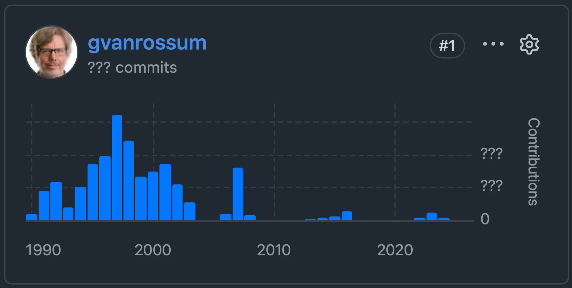
The Python repo has over 130,000 commits made by more than 3,500 contributors over the past 35+ years. The Python core developers are the people with permissions to commit directly to the CPython GitHub repo and plenty of them were at the conference. Out of the following 4 core devs, who were all at the conference, who's made the fewest commits?
- Guido van Rossum, the creator of Python
- Hugo van Kemenade, Python 3.14 and 3.15 release manager
- Łukasz Langa, Python Developer in Residence for ~5 years
- Pablo Galindo Salgado, Python 3.10 and 3.11 release manager
Speaking of commits, how many commits did Guido van Rossum make?
Since we're celebrating 25 years of EuroPython, which of the following expressions does not evaluate to 25?
0x190b110010o3325
3.15 comes with two new built-in functions. Before that, the previous Python version that got new built-ins was 3.10, with also TWO new built-ins. What two built-ins were introduced in 3.10?
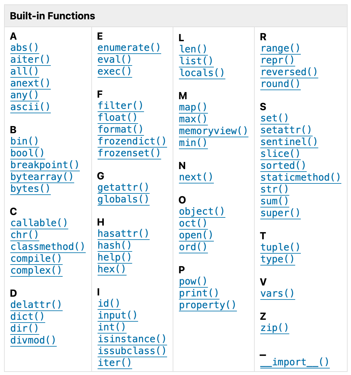
-
aiterandanext -
breakpointandcompile -
frozendictandsentinel -
frozensetandmemoryview
What's printed by the second print if you run this code?
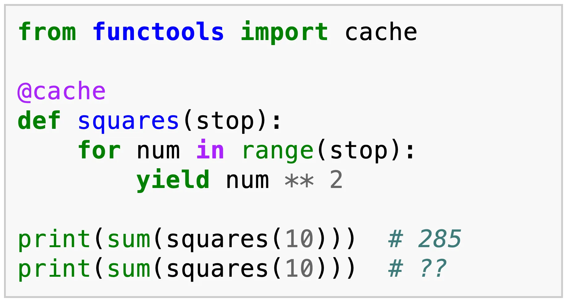
0285KeyErrorValueError
By the way, speaking of commits, do you still remember how many commits Guido van Rossum made?
What does the following cursed Python 2 code print?

'a'25TrueSyntaxError
Explanations
Question 1 — Hosting EuroPython
EuroPython 2009 and 2010 was hosted in Birmingham. EuroPython 2015 and 2016 was hosted in Bilbao. EuroPython 2023, 2024, and 2025 was hosted in Prague. Of the four options, Lisbon is the only European city that never hosted an EuroPython.
Question 2 — poster presentations
Originally, 9 poster presentations were scheduled. After a mixup and a couple cancellations we ended with only 6.
Question 3 — GitHub stars
The official quiz asked you to order all four projects, from most stars to least stars. Can you do it?
On the 15th of July of 2026, this would be the correct ordering:
- FastAPI, 101k
- Django, 88.2k
- uv, 87.5k
- CPython, 73.8k
Question 4 — commits
On the 15th of July of 2026, GitHub reported the following number of all-time...
Python Bytes
#489 Or JSON?
<strong>Topics covered in this episode:</strong><br> <ul> <li><strong><a href="https://adamj.eu/tech/2026/07/15/introducing-django-orjson/?featured_on=pythonbytes">django-orjson</a></strong></li> <li><strong><a href="https://www.peterbe.com/plog/best-django-redis-configuration-for-speed-and-size?featured_on=pythonbytes">Best Django Redis configuration for speed and size</a></strong></li> <li><strong>Linus Torvalds <a href="https://lore.kernel.org/linux-media/CAHk-=wi4zC+Ze8e+p3tMv8TtG_80KzsZ1syL9anBtmEh5Z40vg@mail.gmail.com/?featured_on=pythonbytes">puts the foot down</a> against Anti-AI Kernel Maintainers</strong></li> <li><strong><a href="https://www.djangoproject.com/weblog/2026/jul/15/supporting-the-triptych-project/?featured_on=pythonbytes">Django Steering Council backs the Triptych Project</a></strong></li> <li><strong>Extras</strong></li> <li><strong>Joke</strong></li> </ul><a href='https://www.youtube.com/watch?v=zaoPcuKz970' style='font-weight: bold;'data-umami-event="Livestream-Past" data-umami-event-episode="489">Watch on YouTube</a><br> <p><strong>About the show</strong></p> <p>Sponsored by us! Support our work through:</p> <ul> <li>Our <a href="https://training.talkpython.fm/?featured_on=pythonbytes"><strong>courses at Talk Python</strong></a></li> <li>Consulting from <a href="https://sixfeetup.com/?featured_on=pythonbytes"><strong>Six Feet Up</strong></a></li> </ul> <p><strong>Connect with the hosts</strong></p> <ul> <li>Michael: <a href="https://fosstodon.org/@mkennedy">Mastodon</a> / <a href="https://bsky.app/profile/mkennedy.codes?featured_on=pythonbytes">BlueSky</a> / <a href="https://x.com/mkennedy?featured_on=pythonbytes">X</a> / <a href="https://www.linkedin.com/in/mkennedy/?featured_on=pythonbytes">LinkedIn</a></li> <li>Calvin: <a href="https://sixfeetup.social/@calvin?featured_on=pythonbytes">Mastodon</a> / <a href="https://bsky.app/profile/calvinhp.com?featured_on=pythonbytes">BlueSky</a> / <a href="https://x.com/calvinhp?featured_on=pythonbytes">X</a> / <a href="https://www.linkedin.com/in/calvinhp/?featured_on=pythonbytes">LinkedIn</a></li> <li>Show: <a href="https://fosstodon.org/@pythonbytes">Mastodon</a> / <a href="https://bsky.app/profile/pythonbytes.fm">BlueSky</a> / <a href="https://x.com/PythonBytes?featured_on=pythonbytes">X</a></li> </ul> <p>Join us on YouTube at <a href="https://pythonbytes.fm/stream/live"><strong>pythonbytes.fm/live</strong></a> to be part of the audience. Usually <strong>Tuesday at 7am PT</strong>. Older video versions available there too.</p> <p><strong>Michael #1: <a href="https://adamj.eu/tech/2026/07/15/introducing-django-orjson/?featured_on=pythonbytes">django-orjson</a></strong></p> <ul> <li><strong>Adam Johnson dropped <code>django-orjson</code></strong> - drop-in replacements for the Django and DRF pieces that touch JSON, swapping stdlib <code>json</code> for <strong>orjson</strong>, the Rust-based library. Headline numbers: <strong>10x faster serialization, 2x faster deserialization</strong>.</li> <li><strong>The interesting question is why this needs to be a package at all.</strong> <code>pip install orjson</code> is the easy part. Adam's actual pitch: adopting it "isn't easy, especially when your framework uses <code>json</code> in many different parts." Django scatters JSON across <code>JsonResponse</code>, the test client and test case classes, the <code>json_script</code> template tag, and more. There's no single hook to grab, so you get a library that catches them all.</li> <li><strong>Adam is refreshingly honest about the scale of the win.</strong> His words: <em>"While database queries tend to dominate the typical Django application's runtime, the time spent in serialization and deserialization can still be significant."</em> He calls it <strong>"a nearly free performance win"</strong> - not "this will 10x your app." That's a claim about <em>cost</em>, not magnitude, and it's worth keeping those straight.</li> <li><strong>Worth flagging what the post doesn't cover: caveats.</strong> There are none in the article, but orjson has real ones. Django and Flask both render datetimes as RFC 822 HTTP-date (<code>Wed, 15 Jul 2026 12:00:00 GMT</code>); orjson does ISO 8601. It can't do <code>ensure_ascii</code>, it rejects NaN and Infinity (which stdlib happily emits), and it raises on <code>Decimal</code>. If you've got a JS client parsing dates, that's a wire-format change.</li> <li><strong>Who should actually take this?</strong> If you're a DRF shop shoveling JSON all day, yes - it's cheap and it's real. If your app mostly renders HTML templates, you're optimizing a slice of runtime that's already near zero.</li> <li><strong>The problem Adam's package solves doesn't exist in Flask or Quart.</strong> They already centralize every JSON operation - <code>jsonify</code>, <code>request.get_json()</code>, the test client, the <code>|tojson</code> filter - behind one provider object at <code>app.json</code>. So there's no library to install. It's about ten lines: <div class="codehilite"> <pre><span></span><code><span class="kn">import</span><span class="w"> </span><span class="nn">orjson</span> <span class="kn">from</span><span class="w"> </span><span class="nn">quart.json.provider</span><span class="w"> </span><span class="kn">import</span> <span class="n">JSONProvider</span> <span class="c1"># or flask.json.provider</span> <span class="k">class</span><span class="w"> </span><span class="nc">OrjsonProvider</span><span class="p">(</span><span class="n">JSONProvider</span><span class="p">):</span> <span class="k">def</span><span class="w"> </span><span class="nf">dumps</span><span class="p">(</span><span class="bp">self</span><span class="p">,</span> <span class="n">obj</span><span class="p">,</span> <span class="o">**</span><span class="n">kwargs</span><span class="p">)</span> <span class="o">-></span> <span class="nb">str</span><span class="p">:</span> <span class="k">return</span> <span class="n">orjson</span><span class="o">.</span><span class="n">dumps</span><span class="p">(</span><span class="n">obj</span><span class="p">)</span><span class="o">.</span><span class="n">decode</span><span class="p">()</span> <span class="c1"># provider must return str</span> <span class="k">def</span><span class="w"> </span><span class="nf">loads</span><span class="p">(</span><span class="bp">self</span><span class="p">,</span> <span class="n">s</span><span class="p">,</span> <span class="o">**</span><span class="n">kwargs</span><span class="p">):</span> <span class="k">return</span> <span class="n">orjson</span><span class="o">.</span><span class="n">loads</span><span class="p">(</span><span class="n">s</span><span class="p">)</span> <span class="n">app</span><span class="o">.</span><span class="n">json</span> <span class="o">=</span> <span class="n">OrjsonProvider</span><span class="p">(</span><span class="n">app</span><span class="p">)</span> </code></pre> </div></li> </ul> <p><strong>The numbers on <a href="https://talkpython.fm/?featured_on=pythonbytes">talkpython.fm</a></strong></p> <ul> <li><strong>Evaluated it, measured it, and skipped it.</strong> The biggest JSON payload we serve is our MCP server returning a cached episode transcript, about 139 KB. Swapping the provider saves <strong>0.119 milliseconds per request</strong>. That total response takes 1.1 ms</li> <li><strong>We got 4.1x, not 10x - and the reason is the good lesson.</strong> Payload <em>shape</em> decides your speedup. The 10x is for structure-heavy data, lots of small keys where stdlib burns time in Python-level dispatch per item. Our hot payload is one giant transcript string, so the work is escaping and memcpy</li> </ul> <p><strong>Calvin #2: <a href="https://www.peterbe.com/plog/best-django-redis-configuration-for-speed-and-size?featured_on=pythonbytes">Best Django Redis configuration for speed and size</a></strong></p> <ul> <li>Peter Bengtsson revisits a classic: his 2017 "<a href="https://www.peterbe.com/plog/fastest-redis-optimization-for-django?featured_on=pythonbytes">Fastest Redis configuration for Django</a>" benchmark now has a 2026 update posted this week.</li> <li>The 2017 post pitted django-redis serializers (json, ujson, msgpack, pickle) and compressors (zlib, lzma) against each other; conclusion was <strong>msgpack + zlib</strong> as the sweet spot - avoid the json serializer, it's fat and slow.</li> <li>The 2026 update narrows focus to just compressors: default (no compression), <code>zlib</code>, <code>lzma</code>, and newcomer <code>zstd</code>.</li> <li>New results: <code>lzma</code> compresses best but is slowest; <code>zstd</code> is the fastest compressor on Ubuntu; differences between them are very small.</li> <li>Big takeaway across both: compression buys you a lot of space (2–3.5x smaller) for very little speed cost - worth it for Redis where memory is the constraint.</li> <li>Caveat from the author: results depend heavily on your data - his test stores short strings of numbers, so benchmark your own workload.</li> </ul> <p><strong>Michael #3: Linus Torvalds <a href="https://lore.kernel.org/linux-media/CAHk-=wi4zC+Ze8e+p3tMv8TtG_80KzsZ1syL9anBtmEh5Z40vg@mail.gmail.com/?featured_on=pythonbytes">puts the foot down</a> against Anti-AI Kernel Maintainers</strong></p> <ul> <li>Write up <a href="https://arstechnica.com/ai/2026/07/linus-torvalds-to-critics-of-ai-coding-in-linux-fork-it-or-just-walk-away/?featured_on=pythonbytes">on Ars</a>.</li> <li>Really good coverage by Maximillian: <a href="https://www.youtube.com/watch?v=kxEoF8sn-K4">Time to wake up (for some)</a></li> <li>Torvalds said that “Linux is not one of those anti-AI projects, and if somebody has issues with that, they can do the open-source thing and fork it. Or just walk away.”</li> <li>I agree with Max, putting your head in the sand and waiting for AI to go away will likely mean you won’t be working professionally in software development in the coming years.</li> <li>The statement came amid a lengthy thread arguing about the use of <a href="https://github.com/sashiko-dev/sashiko?featured_on=pythonbytes">Sashiko</a>, an “agentic Linux kernel code review system” that its creators claim can, in tests, independently find 53.6 percent of the bugs that would end up being fixed by human coders in later commits.</li> <li>“We’re not forcing anybody to use [LLM tools], but I will very loudly ignore people who try to argue against other people from using it,” Torvalds said.</li> <li>“Anybody who points to the problems at AI had better be looking in the mirror and pointing at themselves at the same time,” Torvalds wrote.</li> </ul> <p><strong>Calvin #4: <a href="https://www.djangoproject.com/weblog/2026/jul/15/supporting-the-triptych-project/?featured_on=pythonbytes">Django Steering Council backs the Triptych Project</a></strong></p> <ul> <li>Django Steering Council issued a Letter of Collaboration backing Carson Gross & Alex Petros's funding bid for the <a href="https://triptychproject.org/?featured_on=pythonbytes">Triptych Project</a> - three proposals to make HTML more expressive natively, in every browser.</li> <li>The three additions: PUT/PATCH/DELETE methods for forms, button actions (buttons that fire HTTP requests without a wrapping form), and partial page replacement.</li> <li>Distills the core ideas from HTMX/Unpoly/Turbo into the HTML standard itself - no JS, no library, nothing to ship or maintain.</li> <li>Current focus is button actions (<a href="https://github.com/whatwg/html/issues/12330?featured_on=pythonbytes">WHATWG #12330</a>): <code><button action=/logout method=POST>Logout</button></code> instead of wrapping a button in a form.</li> <li>Relevant to Django directly - think the admin submit row and disguised delete links; Django 6.0's template partials were already inspired by these patterns.</li> <li>How to help: companies can send non-binding letters of support on letterhead; individuals can read the proposals and weigh in on the WHATWG issues.</li> </ul> <p><strong>Extras</strong></p> <p>Calvin:</p> <ul> <li><a href="https://github.com/petergpt/doomql?featured_on=pythonbytes">DOOMQL</a> - <strong>A playable first-person shooter whose framebuffer is a SQL query.</strong></li> </ul> <p>Michael:</p> <ul> <li><a href="https://github.com/emmett-framework/granian/releases/tag/v2.7.9?featured_on=pythonbytes"><strong>Granian 2.7.9 fixes WSGI threadpool scheduler starvation/underscaling</strong></a></li> <li><a href="https://talkpython.fm/blog/posts/calvin-hendryx-parker-joins-python-bytes-as-co-host/?featured_on=pythonbytes">Welcome Calvin post</a></li> </ul> <p><strong>Joke: <a href="https://x.com/PR0GRAMMERHUM0R/status/2077211586440151184?featured_on=pythonbytes">Solving all bugs</a></strong></p>
Talk Python Blog
Calvin Hendryx-Parker joins Python Bytes as Co-Host

TL;DR: Calvin Hendryx-Parker is the new permanent co-host of Python Bytes, starting with episode 483 on June 9th, 2026. After almost 10 years, Brian Okken, who founded the show with me back in 2016, has decided it’s time for him to move on.
We have some major news to announce over at Python Bytes. We are welcoming a new co-host to the show: Calvin Hendryx-Parker. After almost 10 years, Brian Okken who founded the show with me, Michael back in 2016 has decided it’s time for him to move on. On the air I called it the next generation of Python Bytes.
July 20, 2026
Wingware
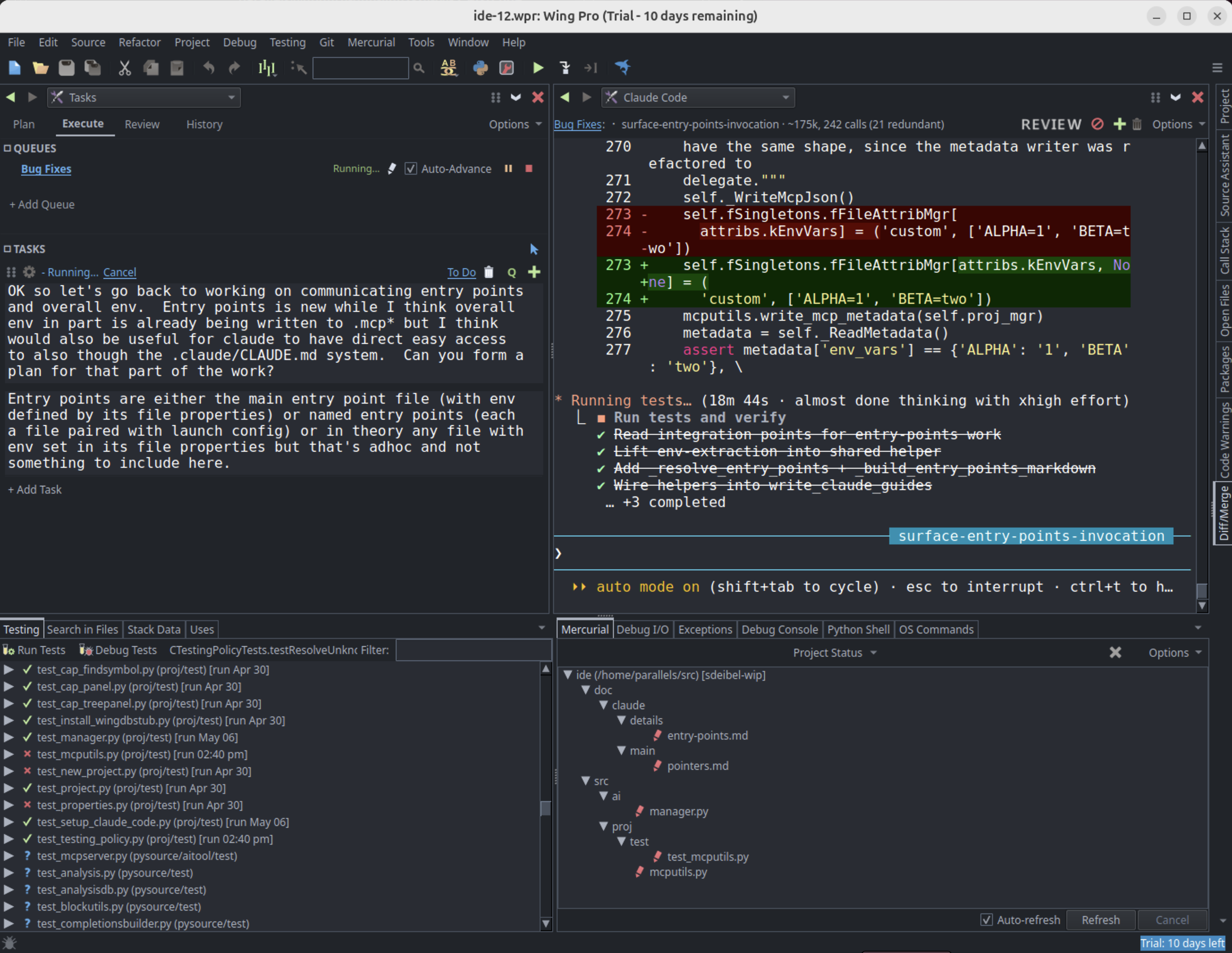
Wing Python IDE Version 12 - July 20, 2026
Wing Python IDE version 12 has been released. Wing 12 integrates the Claude Code AI coding agent directly into the IDE, with a new Claude Code tool, a Tasks tool for planning and reviewing AI agent work, and a set of MCP servers that give the agent access to Wing's source code analysis, unit testing, debugger, and code review features. Wing 12 makes it faster and cheaper to direct AI agents; see our benchmarks for details.
Wing 12 also adds configurable AI-driven Code Actions, code FIX actions, automated Write Tests, pseudo-terminal support for OS Commands and Debug I/O, support for tools and OS Commands in editor splits, a reorganized Tools menu, automatic test discovery, Preferences search, and more.
Downloads
Wing 12 -- the full Python IDE, available as Wing Pro (for agentic development) or Wing Classic (for manual development) depending on your license, with a free 30-day trial of Wing Pro.
Wing 101 v. 12 -- a simplified free Python IDE for teaching beginning programmers.
Wing 11 and earlier versions are not affected by installation of Wing 12 and may be installed and used independently. However, project files for Wing 11 and earlier are converted when opened by Wing 12 and should be saved under a new name, since Wing 12 projects cannot be opened by older versions of Wing.
New in Wing 12
AI Coding Agent Integration with Claude Code
Wing 12 adds a Claude Code tool that integrates the Claude Code AI coding agent with the IDE. Set Up for Claude Code in the Project menu configures the active project for AI agent development.
A set of MCP (Model Context Protocol) servers gives Claude Code access to Wing's source code analysis, testing, and debugger functionality, so the agent can more efficiently navigate and understand your code, write, run, and fix unit tests, and use the debugger to diagnose difficult runtime errors. In our benchmarks, giving Claude Code access to Wing's MCP servers made agent-driven coding tasks both faster and cheaper.
Tasks Tool
The new Tasks tool lets you plan, queue, execute, review, and audit the history of AI agent development tasks, making it easier to supervise and inspect the agent's work before committing it to revision control.
FIX Features and Write Tests
Wing 12 adds AI agent driven FIX features that hand the current debugger bug, failing unit tests, or code warnings to Claude Code for resolution. New Write Tests items in the Testing and editor context menus prompt the agent to write unit tests for selected code.
Code Actions
Wing 12 also adds AI Code Actions, accessed from the FIX icon in the editor toolbar, that operate on selected code or the enclosing scope. Built-in actions include explaining code, reviewing it for quality or security risks, fixing code warnings, optimizing for performance, and updating comments and docstrings. The action list is user-extensible, so you can add your own prompts for tasks you run often.
Pseudo-Terminal for OS Commands and Debug I/O
The OS Commands and Debug I/O tools now default to using a pseudo-terminal that implements full ANSI terminal emulation, so you can run and debug programs that use color output, cursor positioning, or full-screen TUIs.
Redesigned OS Commands Capability
The OS Commands tool has been replaced with configurable OS Commands in the Tools menu. Each OS Command acts like its own tool, for use in any tool or editor split.
Tools in Editor Splits and Reorganized Tools Menu
Tools can now also be added or dragged to editor splits, allowing for much more flexible workspace layout. The Tools menu has been reorganized into related groups, with less-user and legacy tools in an Other sub-menu, so more commonly used tools area easier to find.
Test Discovery and Preferences Search
Wing 12 adds automatic test file discovery and discovery of individual unit tests within files, so you usually don't need to specify test file patterns or add test files individually. The Preferences dialog now supports text search and back/forward navigation.
Other Minor Features and Improvements
Wing 12 also significantly speeds up source code analysis, prompts for SSH passphrases and HTTPS credentials when needed during VCS operations, detects externally modified files much more quickly and with reduced CPU load, saves and restores tool console scrollback across project close/reopen, supports clickable OSC 8 hyperlinks in OS Commands and Debug I/O tools, adds a preference to select the ssh or plink.exe SSH implementation, shows a notice on the next startup when Wing's previous session ended in an unexpected crash, and makes a number of other bug fixes and usability improvements.
Product Line Changes
Wing 12 simplifies the product line. The Commercial / Non-Commercial use distinction has been replaced by two feature-based product tiers:
- Wing Pro -- the full-featured Python IDE including AI agent development tools
- Wing Classic -- the complete traditional Python IDE for hands-on development, with no AI agent features
Anyone may purchase either tier for any purpose. Existing Commercial and Non-Commercial Use licenses both become Wing Pro. Customers who don't need the AI agent features may move to Wing Classic at renewal time, or any time sooner by contacting support@wingware.com.
Wing Personal has been discontinued. Existing Wing Personal users may continue to use Personal 11.x indefinitely, switch to free Wing 101, or purchase a Wing Classic license. See Pricing for details.
Changes and Incompatibilities
The single-LLM-query AI features originally introduced in Wing 11 (the AI Coder and AI Chat tools) are considered legacy in Wing 12 and hidden from the user interface by default. They remain available in projects that already use them and can be re-enabled with Project Properties > AI in Project Properties or in the .``Projects > AI`` preferences.
See Wing's Claude Code Agent Integration for Wing 12's AI agent approach.
If you have questions, please don't hesitate to contact us at support@wingware.com.
July 19, 2026
Paolo Melchiorre
My EuroPython 2026
My EuroPython 2026 experience in Krakow, captured through Mastodon posts about talks, community, people, and moments along the way.
Peter Bengtsson
Best Django Redis configuration for speed and size
`lzma` compresses the most and `zlib` is about as fast as `zstd` in `django_redis` as compressor.
July 18, 2026
PyPy
Moving linux builds to GLIBC==2.28
A short note for visibility.
PyPy builds tarballs of the python interpreter ready for
download. These include the latest
releases and also nightly builds, fresh from our fleet of buildbots. Over the
next couple of days, the nightly builds on linux will transition from
manylinux2014 based docker images to manylinux2_28
images. The practical implication is that
nightly images, and the next releases, will require a minimum of GLIBC>=2.28,
i.e. AlmaLinux8, amanzonlinux 2023, debian 10, ubuntu 20.04. For a good
overview of how this glibc/distro/manylinux all works, see the PEP 600 compliance
page.
The next release will indicate this change by a new PyPy major version, 8.0.0. It should include a Python3.12 interpreter, in which case it will be the last release of the Python 3.11 interpreter.
Core Dispatch
Core Dispatch #8
Welcome back to Core Dispatch! This edition covers July 5 through July 18, 2026. Python 3.15.0 beta 4 landed today, July 18 (we just released it at the EuroPython sprints!), with 3.13.15, 3.14.7 and the first 3.15 release candidate following on August 4.
It's EuroPython week! Much of the core team has been gathered in one place for our annual Language Summit (blog posts to come!) and the conference. Recordings aren't up just yet, but as promised with the PyCon US talks, once they are, we'll pull talks and Language Summit coverage from the team into a future edition.
On the PEP front, discussion is lively: PEP 835
(shorthand syntax for Annotated metadata) and PEP 836
("JIT Go Brrr") are both drawing dozens of new replies, and a few fresh PEPs — including
PEP 840 on name resolution in class namespaces —
have joined the queue.
Don't miss the "One More Thing" at the bottom of this edition. This one's a little sillier (correction: more unhinged) than usual, but we think you'll enjoy it.
As always, if you maintain a package or just like living on the edge, give the final 3.15 beta a spin and file any issues you find.
Upcoming Releases
- Python 3.15.0 beta 4 — Jul 18
- Python 3.13.15 — Aug 04
- Python 3.14.7 — Aug 04
PEP Updates
- PEP 797: Shared Object Proxies
- PEP 838: Adding
python-versiontopyvenv.cfg - PEP 840: Name Resolution in Class Namespaces
Steering Council Updates
Merged PRs
- Add
next_network()to theipaddressmodule - Normalize symlink targets in
tarfile.TarFile.gettarinfo() - Add
tkinter.systray— system tray icon and notifications - Add
tkinter.fontchooser— a font selection dialog - Reject CR and LF in
email.utils.formataddr() - Add a dataclass-like decorator for
ctypesstructures - Stop exposing the internal mapping when comparing
MappingProxyTypeobjects - Fix a data race compiling
string.Templatepatterns in free-threaded builds - Make
tempfile.TemporaryFileWrapperpublic
Discussion
- PEP 835: Shorthand Syntax for
AnnotatedType Metadata — 🔥 36 new replies · 4.6k views - PEP 836: JIT Go Brrr: The Path to a Supported JIT Compiler for CPython — 🔥 28 new replies · 3.9k views
- PEP 840: Name Resolution in Class Namespaces — 🆕 🔥 10 new replies · 496 views
- PEP 822: Dedented Multiline String (d-string) — 7 new replies · 7.6k views
- PEP 832: Virtual Environment Discovery — 6 new replies · 8.8k views
- PEP 827: Type Manipulation — 3 new replies · 8.4k views
- PEP 718: Subscriptable Functions — 3 new replies · 14.3k views
Core Dev Musings
- How to publish to PyPI using GitHub Actions securely — By Brett Cannon
- Security: line goes up — By Hugo van Kemenade
- Fixing the dictionary with Python 3.14 — By Hugo van Kemenade
- EuroPython 2026: Learning from the “not-so-secret” Python security cabal — By Seth Larson
Upcoming CFPs & Conferences
- EuroSciPy 2026 — Jul 18
- PyData PyCon Armenia 2026 — Jul 24
- PyOhio 2026 — Jul 25
- 📋 Plone Conference 2026 Deadline — Aug 01
- 📋 PyCon France 2026 Deadline — Aug 01
- 📋 PyCon Ireland 2026 Deadline — Aug 01
- 📋 PyBay 2026 Deadline — Aug 01
- 📋 PyData Global 2026 Workshop Deadline — Aug 04
One More Thing
"The Meowl is a part of life."
— Ken Jin
"We're just normal men"
— Łukasz Langa
 Pablo during one of his "EuroPython 2026" talks, as hallucinated by AI.
Credits
Python Insider
Python 3.15.0 beta 4 is here!
The final 3.15 beta is out!
July 17, 2026
PyPodcats
Episode 12: With Juanita Gomez
Learn about Juanita Gomez, a Ph.D. candidate at UC Santa Cruz researching open source security. From developing the Spyder IDE to leading community efforts for Scientific Python and singing on stage at SciPy, Juanita shares her journey in open source.Learn about Juanita Gomez, a Ph.D. candidate at UC Santa Cruz researching open source security. From developing the Spyder IDE to leading community efforts for Scientific Python and singing on stage at SciPy, Juanita shares her journey in open source.
We interviewed Juanita Gomez.
Juanita is a Ph.D. candidate in Computer Science at UC Santa Cruz, where her research focuses on improving the security of scientific open source software in collaboration with the Open Source Program Office (OSPO) at UCSC. She is a former developer of the Spyder IDE, and currently one of the community managers for the Scientific Python project. She is also part of the organizing committee for the SciPy conference.
In this episode, Juanita shares how a music YouTube channel led her to open source: the video editing skills she picked up making covers helped her create friendlier documentation, tutorials, and videos for Spyder, which caught the attention of the Scientific Python project founders. She talks about bridging her security research with her passion for open source, and gives practical advice for maintainers who want to make their projects more secure, from GitHub’s built-in security features to the OpenSSF Scorecard. She also opens up about imposter syndrome, being doubly underrepresented as a woman and Latina in tech, and how surrounding herself with people who elevate her work keeps her growing. And yes, there is singing: from auditioning for The X Factor in Colombia as a kid to performing lightning talk songs with the SciPy 5 at the SciPy conference.
Be sure to listen to the episode to learn all about Juanita’s inspiring story!
Topic discussed
- Introductions
- Getting to know Juanita
- How Juanita joined Spyder and made its documentation more friendly
- Reaching new audiences through YouTube tutorials and TikTok
- Joining the Scientific Python project as a community manager
- Her Ph.D. research on open source security at UC Santa Cruz
- Actionable security tips for maintainers: GitHub security features and the OpenSSF Scorecard
- AI and open source security
- Organizing the Scientific Python summits and the SciPy conference
- Imposter syndrome and being a woman and Latina in tech
- Juanita’s music journey, from The X Factor in Colombia to singing at SciPy
Links from the show
- Scientific Python: https://scientific-python.org/
- Spyder IDE: https://www.spyder-ide.org/
- OpenSSF Scorecard: https://scorecard.dev/
- Juanita’s website: https://juanis2112.github.io/
- Juanita’s YouTube channel: https://www.youtube.com/@juanitagomezr
- Spyder YouTube channel: https://www.youtube.com/@SpyderIDE
- Scientific Python TikTok: https://www.tiktok.com/@scientific.python
- Scientific Python YouTube: https://www.youtube.com/@scientific-python
July 16, 2026
Tryton News
Release 1.0.0 of Relatorio
We are proud to announce the release of Relatorio version 1.0.0.
Relatorio is a templating library for OpenDocument using also OpenDocument as source format.
In addition to bug-fixes, this release contains the following improvements:
- Replace python-magic dependency by puremagic
- Remove support for chart template
- Remove support for PDF
The package is available at Client Challenge
The documentation is available at Relatorio — A templating library able to output odt files
1 post - 1 participant
Release 1.0.0 of GooCalendar
We are proud to announce the release 1.0.0 of GooCalendar.
GooCalendar is a Python library that implements a calendar widget for GTK+.
In addition to bug-fixes, this release contains this following improvements:
- Remove GooCanvas dependency
- Remove support for Python older than 3.9
- Upgrade to pyproject
GooCalendar is available on PyPI: GooCalendar · PyPI
The documentation is available at goocalendar — Calendar widget — A calendar widget for GTK
1 post - 1 participant
Seth Michael Larson
EuroPython 2026: Learning from the “not-so-secret” Python security cabal
I delivered this talk at EuroPython 2026, I'll update this blog post once the recording is available on EuroPython's YouTube channel. Below are the slides and full list of links and resources included. This talk is a continuation of a talk I gave a year ago: “Security Work isn’t Special” as the keynote for OpenSSF Community Day NA where I lamented on how security work didn't match other Open Source contribution models like documentation, community, or code contributions.
My work as the Security Developer-in-Residence at the Python Software Foundation is sponsored by Alpha-Omega. Thanks to Alpha-Omega for supporting security in the Python ecosystem.
Links and Resources
- Slides
- Python Software Foundation Blog
- Python Insider Blog
- Security Work isn’t Special
- Security Line Goes Up by Hugo van Kemenade
- Vulnerability Reports are not special anymore by Filippo Valsorda
- LLM generated vulnerabilities by Linus Torvalds
- Python Security Policy and Threat Model
- Python Security Response Team
- PEP 811 - Defining Python Security Response Team membership and responsibilities
Thanks for reading ♥ I would love to hear your thoughts! Contact me via Mastodon, Bluesky, or email. Browse the blog archive. Check out my blogroll.
July 15, 2026
Python Software Foundation
Affirm Your PSF Membership Voting Status
Every Python Software Foundation (PSF) voting-eligible Member (Supporting, Contributing, and Fellow) needs to affirm their membership to vote in this year’s PSF Board and Python Packaging Council (PPC) elections.
If you wish to vote in either the PSF Board or Python Packaging Council elections, you must affirm your intention to vote for each election no later than Tuesday, August 25th, 2:00 pm UTC, to participate in this year’s elections. This year’s election votes begin Tuesday, September 1st, 2:00 pm UTC, and close on Tuesday, September 15th, 2:00 pm UTC.
Election communications from psfmember.org
You should have received an email from "psf@psfmember.org <Python Software Foundation>" with the subject "[Action Required] Affirm your PSF Membership voting intention for the 2026 PSF Board Election" and/or “2026 Python Packaging Council Inaugural Election Information & Schedule” that contains information on how to affirm your voting status. If you were expecting to receive the email but have not (make sure to check your spam!), please email psf-elections@pyfound.org for the PSF Board election or pc-elections@python.org, and we’ll assist you. Please note: If you opted out of emails related to your membership, you did not receive these emails.
PSF Members should review their communication preferences on psfmember.org if you would like to opt in or out of receiving emails about the PSF Board, PPC elections, or both. Here’s how:
- Login to psfmember.org
- Navigate to your “Profile” page
- Click the “Name and Address” tab
- Scroll down, designate your preferences
- Click submit
If you had previously opted out of communications from the PSF through psfmember.org and would like to review or change your preference, we encourage you to update them using the instructions above. The PSF only sends a handful of election and fundraising related communications every year via psfmember.org. The PSF newsletter runs through a separate mailing list (and we welcome you to sign up!).
How to affirm your intention to vote
You can affirm your voting intention by following the steps in our video tutorial:
- Log in to psfmember.org
- Choose “Your Memberships” page at the top right to check your eligibility to vote (You must be a Contributing, Supporting, or Fellow member)
- Choose “Voting Affirmation” page at the top right
- Select your preferred intention for voting in 2026 (which now includes a second affirmation regarding your intention to vote in the Python Packaging Council election)
- Click the “Submit” button
Need to check your membership status?
Log on to psfmember.org and visit your PSF Member User Information page to see your membership record and status. If you are a voting-eligible member (active Supporting, Contributing, and Fellow members of the PSF) and do not already have a login, please create an account on psfmember.org and then email psf-elections@pyfound.org so we can link your membership to your account. Please ensure you have an account linked to your membership so that we can have the most up-to-date contact information for you in the future.
PSF Bylaws
Section 4.2 of the PSF Bylaws requires that “Members of any membership class with voting rights must affirm each year to the corporation in writing that such member intends to be a voting member for such year.”
Our motivation is to ensure that our elections can meet quorum as required by Section 3.9 of our bylaws. As our membership has grown, we have seen that an increasing number of Contributing and Fellow members with indefinite membership do not engage with our annual election, making quorum difficult to reach.
An election that does not reach quorum is invalid. This would cause the whole voting process to be re-held, resulting in fewer voters and an undue amount of effort on the part of the PSF Staff.
Reminders about membership and voting
Reminder: If you were formerly a Managing member, your membership type was changed last year to Contributing per 2024’s Bylaw change that merged Managing and Contributing memberships.
Per another recent Bylaw change that allows for simplifying the voter affirmation process by treating past voting activity as intent to continue voting, if you voted last year, you will automatically be added to the 2026 voter roll. Please note: If you removed or changed your email on psfmember.org, you may not automatically be added to this year's voter roll.
What happens next?
You’ll get an email from OpaVote with a ballot (or two!) on or right before September 1st, and then you can vote!
Check out our PSF Membership page to learn more. If you have questions about membership, nominations, or this year’s Board election, please email psf-elections@pyfound.org or join the PSF Discord for the upcoming Board Office Hours on August 11th, 9 PM UTC. You are also welcome to join the discussion about the PSF Board election on the Python Discuss forum.
Django Weblog
Supporting the Triptych Project
The Django Steering Council — in its role as the DSF's arm for technical governance — has provided a Letter of Collaboration in support of a funding application by Carson Gross and Alex Petros to advance the Triptych Project: three proposals to make HTML itself more expressive, in every browser, by default.
Here's why, and how you can help.
HTML over the wire, and Django
The last few years have seen a move back towards serving multipage applications, with server-rendered templates. The HTMX library has probably had the biggest impact in the Django space, but Unpoly, Turbo, and others are part of the same story: send HTML over the wire, let the browser do what browsers do, and skip the client-side application layer where you don't really need it. It's a simpler model of the web — and it's one that speaks to Django's heart.
This isn't a movement Django has watched from the sidelines. Template partials, added in Django 6.0, were directly inspired by the patterns these libraries make natural.
The Triptych Project
The Triptych Project takes the core insights from HTMX (and the related libraries) and proposes them for the HTML standard itself. Three small additions:
- PUT, PATCH, and DELETE methods for forms — completing HTML's HTTP vocabulary.
- Button actions — buttons that make HTTP requests without a wrapping form. This is the current focus.
- Partial page replacement — links, forms, and buttons that target part of the DOM.
Together these aim to make it possible to build far more of the web with plain HTML — no JavaScript dependency, no library, nothing to ship or maintain.
Button actions
The current proposal (WHATWG #12330, full proposal) adds the action and method attributes to <button>. The canonical example is logout. Today there's no semantic way to write a logout button; you have to wrap it in a form:
<form action=/logout method=POST>
  <button>Logout</button>
</form>
Every Django developer has written this kind of thing. With button actions we could write the simpler single line:
<button action=/logout method=POST>Logout</button>
This isn't abstract for us. The Django admin's submit row holds multiple buttons, and a link disguised as a button:
<div class="submit-row">
  <input type="submit" value="Save" class="default" name="_save">
  <input type="submit" value="Save and add another" name="_addanother">
  <input type="submit" value="Save and continue editing" name="_continue">
  <a href="/admin/auth/user/.../delete/" class="deletelink">Delete</a>
</div>
Here, all the save inputs lead to the same action URL from the wrapping form. The view then branches on the submitted name value. That, of course, works, but we can imagine simpler, more flexible ideas being enabled via the Multi-Action Pages examples in the proposal.
The disguised submit link leads to the deletion confirmation page, where we then submit a form to confirm the action. That's the correct behaviour, but the markup confuses the intent: this isn't (really) a navigation to a new page, it's the first step of an action — deleting the object. The proposal's discussion of Buttons vs Links describes situations we come up against writing applications regularly.
The goal here is simpler patterns that will help us write better markup.
Why we're supporting this
The Django Software Foundation's mission includes a commitment to "advance the state of the art in Web development". Standards work is that in its purest form: an improvement to HTML lands for everyone, in every framework, in every browser, indefinitely.
It's also slow, painstaking work — specification, implementer engagement, web platform tests — that needs sustained attention. Carson and Alex are applying for funds so that people can devote real time to it. Our Letter of Collaboration is a concrete contribution to that application.
How you can help
If your company builds on Django, or indeed any other framework — with HTMX, Unpoly, Turbo, or plain HTML forms — this work benefits you directly. Carson and Alex are seeking non-binding letters of support on official letterhead for the funding application. Details and contacts are on the Triptych Project site.
Individually, do read the proposals, weigh in constructively on the WHATWG issues, and spread the word.
A simpler web is a better web. We're glad to support work that moves HTML in that direction.